Application of differentiations in neural networks

Last Updated on March 16, 2023

Differential calculus is a crucial instrument in machine learning algorithms. Neural networks particularly, the gradient descent algorithm relies upon upon the gradient, which is a quantity computed by differentiation.

In this tutorial, we’re going to see how the back-propagation method is utilized in discovering the gradients in neural networks.

After ending this tutorial, you may know

• What is a whole differential and full by-product
• How to compute the complete derivatives in neural networks
• How back-propagation helped in computing the complete derivatives

Let’s get started

Application of differentiations in neural networks
Photo by Freeman Zhou, some rights reserved.

Tutorial overview

This tutorial is break up into 5 components; they’re:

1. Total differential and full derivatives
2. Algebraic illustration of a multilayer perceptron model
3. Finding the gradient by back-propagation
4. Matrix sort of gradient equations
5. Implementing back-propagation

Total differential and full derivatives

For a carry out resembling $f(x)$, we title denote its by-product as $f'(x)$ or $frac{df}{dx}$. But for a multivariate carry out, resembling $f(u,v)$, we have a partial by-product of $f$ with respect to $u$ denoted as $frac{partial f}{partial u}$, or sometimes written as $f_u$. A partial by-product is obtained by differentiation of $f$ with respect to $u$ whereas assuming the alternative variable $v$ is a unbroken. Therefore, we use $partial$ as an alternative of $d$ as a result of the picture for differentiation to counsel the excellence.

However, what if the $u$ and $v$ in $f(u,v)$ are every carry out of $x$? In completely different phrases, we’ll write $u(x)$ and $v(x)$ and $f(u(x), v(x))$. So $x$ determines the price of $u$ and $v$ and in flip, determines $f(u,v)$. In this case, it is utterly great to ask what’s $frac{df}{dx}$, as $f$ is finally determined by $x$.

This is the thought of full derivatives. In reality, for a multivariate carry out $f(t,u,v)=f(t(x),u(x),v(x))$, we always have
$$
frac{df}{dx} = frac{partial f}{partial t}frac{dt}{dx} + frac{partial f}{partial u}frac{du}{dx} + frac{partial f}{partial v}frac{dv}{dx}
$$
The above notation is known as the complete by-product because of it is sum of the partial derivatives. In essence, it is making use of chain rule to hunt out the differentiation.

If we take away the $dx$ half throughout the above equation, what we get is an approximate change in $f$ with respect to $x$, i.e.,
$$
df = frac{partial f}{partial t}dt + frac{partial f}{partial u}du + frac{partial f}{partial v}dv
$$
We title this notation the complete differential.

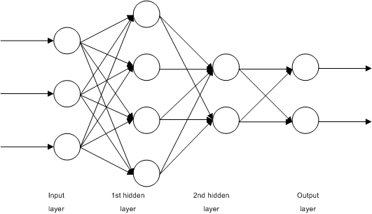
Algebraic illustration of a multilayer perceptron model

Consider the neighborhood:

An occasion of neural neighborhood. Source: https://commons.wikimedia.org/wiki/File:Multilayer_Neural_Network.png

This is a straightforward, fully-connected, 4-layer neural neighborhood. Let’s title the enter layer as layer 0, the two hidden layers the layer 1 and a pair of, and the output layer as layer 3. In this picture, we see that we have $n_0=3$ enter fashions, and $n_1=4$ fashions throughout the first hidden layer and $n_2=2$ fashions throughout the second enter layer. There are $n_3=2$ output fashions.

If we denote the enter to the neighborhood as $x_i$ the place $i=1,cdots,n_0$ and the neighborhood’s output as $hat{y}_i$ the place $i=1,cdots,n_3$. Then we’ll write

$$
begin{aligned}
h_{1i} &= f_1(sum_{j=1}^{n_0} w^{(1)}_{ij} x_j + b^{(1)}_i) & textual content material{for } i &= 1,cdots,n_1
h_{2i} &= f_2(sum_{j=1}^{n_1} w^{(2)}_{ij} h_{1j} + b^{(2)}_i) & i &= 1,cdots,n_2
hat{y}_i &= f_3(sum_{j=1}^{n_2} w^{(3)}_{ij} h_{2j} + b^{(3)}_i) & i &= 1,cdots,n_3
end{aligned}
$$

Here the activation carry out at layer $i$ is denoted as $f_i$. The outputs of first hidden layer are denoted as $h_{1i}$ for the $i$-th unit. Similarly, the outputs of second hidden layer are denoted as $h_{2i}$. The weights and bias of unit $i$ in layer $okay$ are denoted as $w^{(okay)}_{ij}$ and $b^{(okay)}_i$ respectively.

In the above, we’ll see that the output of layer $k-1$ will feed into layer $okay$. Therefore, whereas $hat{y}_i$ is expressed as a carry out of $h_{2j}$, nonetheless $h_{2i}$ may also be a carry out of $h_{1j}$ and in flip, a carry out of $x_j$.

The above describes the event of a neural neighborhood by the use of algebraic equations. Training a neural neighborhood would want to specify a *loss carry out* as successfully so we’ll lower it throughout the teaching loop. Depends on the making use of, we typically use cross entropy for categorization points or indicate squared error for regression points. With the purpose variables as $y_i$, the indicate sq. error loss carry out is specified as
$$
L = sum_{i=1}^{n_3} (y_i-hat{y}_i)^2
$$

Want to Get Started With Calculus for Machine Learning?

Take my free 7-day e mail crash course now (with sample code).

Click to sign-up and as well as get a free PDF Ebook mannequin of the course.

Finding the gradient by back-propagation

In the above assemble, $x_i$ and $y_i$ are from the dataset. The parameters to the neural neighborhood are $w$ and $b$. While the activation options $f_i$ are by design the outputs at each layer $h_{1i}$, $h_{2i}$, and $hat{y}_i$ are dependent variables. In teaching the neural neighborhood, our purpose is to exchange $w$ and $b$ in each iteration, notably, by the gradient descent change rule:
$$
begin{aligned}
w^{(okay)}_{ij} &= w^{(okay)}_{ij} – eta frac{partial L}{partial w^{(okay)}_{ij}}
b^{(okay)}_{i} &= b^{(okay)}_{i} – eta frac{partial L}{partial b^{(okay)}_{i}}
end{aligned}
$$
the place $eta$ is the academic worth parameter to gradient descent.

From the equation of $L$ everyone knows that $L$ is not going to be relying on $w^{(okay)}_{ij}$ or $b^{(okay)}_i$ nonetheless on $hat{y}_i$. However, $hat{y}_i$ can be written as carry out of $w^{(okay)}_{ij}$ or $b^{(okay)}_i$ finally. Let’s see one after the opposite how the weights and bias at layer $okay$ can be associated to $hat{y}_i$ on the output layer.

We begin with the loss metric. If we take into consideration the dearth of a single information stage, we have
$$
begin{aligned}
L &= sum_{i=1}^{n_3} (y_i-hat{y}_i)^2
frac{partial L}{partial hat{y}_i} &= 2(y_i – hat{y}_i) & textual content material{for } i &= 1,cdots,n_3
end{aligned}
$$
Here we see that the loss carry out relies upon upon all outputs $hat{y}_i$ and resulting from this reality we’ll uncover a partial by-product $frac{partial L}{partial hat{y}_i}$.

Now let’s check out the output layer:
$$
begin{aligned}
hat{y}_i &= f_3(sum_{j=1}^{n_2} w^{(3)}_{ij} h_{2j} + b^{(3)}_i) & textual content material{for }i &= 1,cdots,n_3
frac{partial L}{partial w^{(3)}_{ij}} &= frac{partial L}{partial hat{y}_i}frac{partial hat{y}_i}{partial w^{(3)}_{ij}} & i &= 1,cdots,n_3; j=1,cdots,n_2
&= frac{partial L}{partial hat{y}_i} f’_3(sum_{j=1}^{n_2} w^{(3)}_{ij} h_{2j} + b^{(3)}_i)h_{2j}
frac{partial L}{partial b^{(3)}_i} &= frac{partial L}{partial hat{y}_i}frac{partial hat{y}_i}{partial b^{(3)}_i} & i &= 1,cdots,n_3
&= frac{partial L}{partial hat{y}_i}f’_3(sum_{j=1}^{n_2} w^{(3)}_{ij} h_{2j} + b^{(3)}_i)
end{aligned}
$$
Because the burden $w^{(3)}_{ij}$ at layer 3 applies to enter $h_{2j}$ and impacts output $hat{y}_i$ solely. Hence we’ll write the by-product $frac{partial L}{partial w^{(3)}_{ij}}$ as a result of the product of two derivatives $frac{partial L}{partial hat{y}_i}frac{partial hat{y}_i}{partial w^{(3)}_{ij}}$. Similar case for the bias $b^{(3)}_i$ as successfully. In the above, we make use of $frac{partial L}{partial hat{y}_i}$, which we already derived beforehand.

But in reality, we’ll moreover write the partial by-product of $L$ with respect to output of second layer $h_{2j}$. It is not going to be used for the change of weights and bias on layer 3 nonetheless we’re going to see its significance later:
$$
begin{aligned}
frac{partial L}{partial h_{2j}} &= sum_{i=1}^{n_3}frac{partial L}{partial hat{y}_i}frac{partial hat{y}_i}{partial h_{2j}} & textual content material{for }j &= 1,cdots,n_2
&= sum_{i=1}^{n_3}frac{partial L}{partial hat{y}_i}f’_3(sum_{j=1}^{n_2} w^{(3)}_{ij} h_{2j} + b^{(3)}_i)w^{(3)}_{ij}
end{aligned}
$$
This one is the attention-grabbing one and completely completely different from the sooner partial derivatives. Note that $h_{2j}$ is an output of layer 2. Each and every output in layer 2 will impact the output $hat{y}_i$ in layer 3. Therefore, to hunt out $frac{partial L}{partial h_{2j}}$ now we have so as to add up every output at layer 3. Thus the summation sign throughout the equation above. And we’ll take into consideration $frac{partial L}{partial h_{2j}}$ as the complete by-product, by which we utilized the chain rule $frac{partial L}{partial hat{y}_i}frac{partial hat{y}_i}{partial h_{2j}}$ for every output $i$ after which sum them up.

If we switch once more to layer 2, we’ll derive the derivatives equally:
$$
begin{aligned}
h_{2i} &= f_2(sum_{j=1}^{n_1} w^{(2)}_{ij} h_{1j} + b^{(2)}_i) & textual content material{for }i &= 1,cdots,n_2
frac{partial L}{partial w^{(2)}_{ij}} &= frac{partial L}{partial h_{2i}}frac{partial h_{2i}}{partial w^{(2)}_{ij}} & i&=1,cdots,n_2; j=1,cdots,n_1
&= frac{partial L}{partial h_{2i}}f’_2(sum_{j=1}^{n_1} w^{(2)}_{ij} h_{1j} + b^{(2)}_i)h_{1j}
frac{partial L}{partial b^{(2)}_i} &= frac{partial L}{partial h_{2i}}frac{partial h_{2i}}{partial b^{(2)}_i} & i &= 1,cdots,n_2
&= frac{partial L}{partial h_{2i}}f’_2(sum_{j=1}^{n_1} w^{(2)}_{ij} h_{1j} + b^{(2)}_i)
frac{partial L}{partial h_{1j}} &= sum_{i=1}^{n_2}frac{partial L}{partial h_{2i}}frac{partial h_{2i}}{partial h_{1j}} & j&= 1,cdots,n_1
&= sum_{i=1}^{n_2}frac{partial L}{partial h_{2i}}f’_2(sum_{j=1}^{n_1} w^{(2)}_{ij} h_{1j} + b^{(2)}_i) w^{(2)}_{ij}
end{aligned}
$$

In the equations above, we’re reusing $frac{partial L}{partial h_{2i}}$ that we derived earlier. Again, this by-product is computed as a sum of a lot of merchandise from the chain rule. Also very like the sooner, we derived $frac{partial L}{partial h_{1j}}$ as successfully. It is not going to be used to teach $w^{(2)}_{ij}$ nor $b^{(2)}_i$ nonetheless will in all probability be used for the layer prior. So for layer 1, we have

$$
begin{aligned}
h_{1i} &= f_1(sum_{j=1}^{n_0} w^{(1)}_{ij} x_j + b^{(1)}_i) & textual content material{for } i &= 1,cdots,n_1
frac{partial L}{partial w^{(1)}_{ij}} &= frac{partial L}{partial h_{1i}}frac{partial h_{1i}}{partial w^{(1)}_{ij}} & i&=1,cdots,n_1; j=1,cdots,n_0
&= frac{partial L}{partial h_{1i}}f’_1(sum_{j=1}^{n_0} w^{(1)}_{ij} x_j + b^{(1)}_i)x_j
frac{partial L}{partial b^{(1)}_i} &= frac{partial L}{partial h_{1i}}frac{partial h_{1i}}{partial b^{(1)}_i} & i&=1,cdots,n_1
&= frac{partial L}{partial h_{1i}}f’_1(sum_{j=1}^{n_0} w^{(1)}_{ij} x_j + b^{(1)}_i)
end{aligned}
$$

and this completes all the derivatives needed for teaching of the neural neighborhood using gradient descent algorithm.

Recall how we derived the above: We first start from the loss carry out $L$ and uncover the derivatives one after the opposite throughout the reverse order of the layers. We write down the derivatives on layer $okay$ and reuse it for the derivatives on layer $k-1$. While computing the output $hat{y}_i$ from enter $x_i$ begins from layer 0 forward, computing gradients are throughout the reversed order. Hence the determine “back-propagation”.

Matrix sort of gradient equations

While we did not use it above, it is cleaner to put in writing down the equations in vectors and matrices. We can rewrite the layers and the outputs as:
$$
mathbf{a}_k = f_k(mathbf{z}_k) = f_k(mathbf{W}_kmathbf{a}_{k-1}+mathbf{b}_k)
$$
the place $mathbf{a}_k$ is a vector of outputs of layer $okay$, and assume $mathbf{a}_0=mathbf{x}$ is the enter vector and $mathbf{a}_3=hat{mathbf{y}}$ is the output vector. Also denote $mathbf{z}_k = mathbf{W}_kmathbf{a}_{k-1}+mathbf{b}_k$ for consolation of notation.

Under such notation, we’ll signify $frac{partial L}{partialmathbf{a}_k}$ as a vector (so that of $mathbf{z}_k$ and $mathbf{b}_k$) and $frac{partial L}{partialmathbf{W}_k}$ as a matrix. And then if $frac{partial L}{partialmathbf{a}_k}$ is assumed, we have
$$
begin{aligned}
frac{partial L}{partialmathbf{z}_k} &= frac{partial L}{partialmathbf{a}_k}odot f_k'(mathbf{z}_k)
frac{partial L}{partialmathbf{W}_k} &= left(frac{partial L}{partialmathbf{z}_k}correct)^prime cdot mathbf{a}_k
frac{partial L}{partialmathbf{b}_k} &= frac{partial L}{partialmathbf{z}_k}
frac{partial L}{partialmathbf{a}_{k-1}} &= left(frac{partialmathbf{z}_k}{partialmathbf{a}_{k-1}}correct)^topcdotfrac{partial L}{partialmathbf{z}_k} = mathbf{W}_k^topcdotfrac{partial L}{partialmathbf{z}_k}
end{aligned}
$$
the place $frac{partialmathbf{z}_k}{partialmathbf{a}_{k-1}}$ is a Jacobian matrix as every $mathbf{z}_k$ and $mathbf{a}_{k-1}$ are vectors, and this Jacobian matrix happens to be $mathbf{W}_k$.

Implementing back-propagation

We need the matrix sort of equations because of it may well make our code simpler and averted various loops. Let’s see how we’ll convert these equations into code and make a multilayer perceptron model for classification from scratch using numpy.

The very very first thing now we have to implement the activation carry out and the loss carry out. Both needs to be differentiable options or in another case our gradient descent course of would not work. Nowadays, it’s normal to utilize ReLU activation throughout the hidden layers and sigmoid activation throughout the output layer. We define them as a carry out (which assumes the enter as numpy array) along with their differentiation:

import numpy as np</p><p># Find a small float to avoid division by zero<br />epsilon = np.finfo(float).eps</p><p># Sigmoid carry out and its differentiation<br />def sigmoid(z):<br /> return 1/(1+np.exp(-z.clip(-500, 500)))<br />def dsigmoid(z):<br /> s = sigmoid(z)<br /> return 2 * s * (1-s)</p><p># ReLU carry out and its differentiation<br />def relu(z):<br /> return np.most(0, z)<br />def drelu(z):<br /> return (z > 0).astype(float)

1 2 3 4 5 6 7 8 9 10 11 12 13 14 15 16 17

import numpy as np   # Find a small float to avoid division by zero epsilon = np.finfo(float).eps   # Sigmoid carry out and its differentiation def sigmoid(z):     return 1/(1+np.exp(–z.clip(–500, 500))) def dsigmoid(z):     s = sigmoid(z)     return 2 * s * (1–s)   # ReLU carry out and its differentiation def relu(z):     return np.most(0, z) def drelu(z):     return (z > 0).astype(float)

We deliberately clip the enter of the sigmoid carry out to between -500 to +500 to avoid overflow. Otherwise, these options are trivial. Then for classification, we care about accuracy nonetheless the accuracy carry out is not going to be differentiable. Therefore, we use the cross entropy carry out as loss for teaching:

# Loss carry out L(y, yhat) and its differentiation<br />def cross_entropy(y, yhat):<br /> “””Binary cross entropy carry out<br /> L = – y log yhat – (1-y) log (1-yhat)</p><p> Args:<br /> y, yhat (np.array): 1xn matrices which n are the number of information conditions<br /> Returns:<br /> frequent cross entropy price of type 1×1, averaging over the n conditions<br /> “””<br /> return -(y.T @ np.log(yhat.clip(epsilon)) + (1-y.T) @ np.log((1-yhat).clip(epsilon))) / y.type[1]</p><p>def d_cross_entropy(y, yhat):<br /> “”” dL/dyhat “””<br /> return – np.divide(y, yhat.clip(epsilon)) + np.divide(1-y, (1-yhat).clip(epsilon))

1 2 3 4 5 6 7 8 9 10 11 12 13 14 15

# Loss carry out L(y, yhat) and its differentiation def cross_entropy(y, yhat):     “”“Binary cross entropy carry out         L = – y log yhat – (1-y) log (1-yhat)       Args:         y, yhat (np.array): 1xn matrices which n are the number of information conditions     Returns:         frequent cross entropy price of type 1×1, averaging over the n conditions     ““”     return –(y.T @ np.log(yhat.clip(epsilon)) + (1–y.T) @ np.log((1–yhat).clip(epsilon))) / y.type[1]   def d_cross_entropy(y, yhat):     “”” dL/dyhat ““”     return – np.divide(y, yhat.clip(epsilon)) + np.divide(1–y, (1–yhat).clip(epsilon))

In the above, we assume the output and the purpose variables are row matrices in numpy. Hence we use the dot product operator @ to compute the sum and divide by the number of parts throughout the output. Note that this design is to compute the frequent cross entropy over a batch of samples.

Then we’ll implement our multilayer perceptron model. To make it less complicated to study, we have to create the model by providing the number of neurons at each layer along with the activation carry out on the layers. But on the same time, we would moreover need the differentiation of the activation options along with the differentiation of the loss carry out for the teaching. The loss carry out itself, nonetheless, is not going to be required nonetheless useful for us to hint the progress. We create a class to ensapsulate your complete model, and description each layer $okay$ in response to the parts:
$$
mathbf{a}_k = f_k(mathbf{z}_k) = f_k(mathbf{a}_{k-1}mathbf{W}_k+mathbf{b}_k)
$

class mlp:<br /> ”’Multilayer perceptron using numpy<br /> ”’<br /> def __init__(self, layersizes, activations, derivatives, lossderiv):<br /> “””keep in mind config, then initialize array to hold NN parameters with out init”””<br /> # preserve NN config<br /> self.layersizes = layersizes<br /> self.activations = activations<br /> self.derivatives = derivatives<br /> self.lossderiv = lossderiv<br /> # parameters, each is a 2D numpy array<br /> L = len(self.layersizes)<br /> self.z = [None] * L<br /> self.W = [None] * L<br /> self.b = [None] * L<br /> self.a = [None] * L<br /> self.dz = [None] * L<br /> self.dW = [None] * L<br /> self.db = [None] * L<br /> self.da = [None] * L</p><p> def initialize(self, seed=42):<br /> np.random.seed(seed)<br /> sigma = 0.1<br /> for l, (insize, outsize) in enumerate(zip(self.layersizes, self.layersizes[1:]), 1):<br /> self.W[l] = np.random.randn(insize, outsize) * sigma<br /> self.b[l] = np.random.randn(1, outsize) * sigma</p><p> def forward(self, x):<br /> self.a[0] = x<br /> for l, func in enumerate(self.activations, 1):<br /> # z = W a + b, with `a` as output from earlier layer<br /> # `W` is of dimension rxs and `a` the dimensions sxn with n the number of information conditions, `z` the dimensions rxn<br /> # `b` is rx1 and broadcast to each column of `z`<br /> self.z[l] = (self.a[l-1] @ self.W[l]) + self.b[l]<br /> # a = g(z), with `a` as output of this layer, of dimension rxn<br /> self.a[l] = func(self.z[l])<br /> return self.a[-1]

1 2 3 4 5 6 7 8 9 10 11 12 13 14 15 16 17 18 19 20 21 22 23 24 25 26 27 28 29 30 31 32 33 34 35 36 37 38

class mlp:     ”‘Multilayer perceptron using numpy     ‘”     def __init__(self, layersizes, activations, derivatives, lossderiv):         “”“keep in mind config, then initialize array to hold NN parameters with out init”“”         # preserve NN config         self.layersizes = layersizes         self.activations = activations         self.derivatives = derivatives         self.lossderiv = lossderiv         # parameters, each is a 2D numpy array         L = len(self.layersizes)         self.z = [None] * L         self.W = [None] * L         self.b = [None] * L         self.a = [None] * L         self.dz = [None] * L         self.dW = [None] * L         self.db = [None] * L         self.da = [None] * L       def initialize(self, seed=42):         np.random.seed(seed)         sigma = 0.1         for l, (insize, outsize) in enumerate(zip(self.layersizes, self.layersizes[1:]), 1):             self.W[l] = np.random.randn(insize, outsize) * sigma             self.b[l] = np.random.randn(1, outsize) * sigma       def forward(self, x):         self.a[0] = x         for l, func in enumerate(self.activations, 1):             # z = W a + b, with `a` as output from earlier layer             # `W` is of dimension rxs and `a` the dimensions sxn with n the number of information conditions, `z` the dimensions rxn             # `b` is rx1 and broadcast to each column of `z`             self.z[l] = (self.a[l–1] @ self.W[l]) + self.b[l]             # a = g(z), with `a` as output of this layer, of dimension rxn             self.a[l] = func(self.z[l])         return self.a[–1]

The variables on this class z, W, b, and a are for the forward cross and the variables dz, dW, db, and da are their respective gradients that to be computed throughout the back-propagation. All these variables are supplied as numpy arrays.

As we’re going to see later, we’ll examine our model using information generated by scikit-learn. Hence we’re going to see our information in numpy array of type “(number of samples, number of features)”. Therefore, each sample is obtainable as a row on a matrix, and in carry out forward(), the burden matrix is right-multiplied to each enter a to the layer. While the activation carry out and dimension of each layer can be completely completely different, the tactic is analogous. Thus we transform the neural neighborhood’s enter x to its output by a loop throughout the forward() carry out. The neighborhood’s output is solely the output of the ultimate layer.

To follow the neighborhood, now we have to run the back-propagation after each forward cross. The back-propagation is to compute the gradient of the burden and bias of each layer, starting from the output layer to the enter layer. With the equations we derived above, the back-propagation carry out is carried out as:

The solely distinction proper right here is that we compute db not for one teaching sample, nonetheless to your complete batch. Since the loss carry out is the cross entropy averaged all through the batch, we compute db moreover by averaging all through the samples.

Up to proper right here, we completed our model. The change() carry out merely applies the gradients found by the back-propagation to the parameters W and b using the gradient descent change rule.

To try our model, we make use of scikit-learn to generate a classification dataset:

from sklearn.datasets import make_circles<br />from sklearn.metrics import accuracy_score</p><p># Make information: Two circles on x-y plane as a classification disadvantage<br />X, y = make_circles(n_samples=1000, subject=0.5, noise=0.1)<br />y = y.reshape(-1,1) # our model expects a 2D array of (n_sample, n_dim)

1 2 3 4 5 6

from sklearn.datasets import make_circles from sklearn.metrics import accuracy_score   # Make information: Two circles on x-y plane as a classification disadvantage X, y = make_circles(n_samples=1000, subject=0.5, noise=0.1) y = y.reshape(–1,1) # our model expects a 2D array of (n_sample, n_dim)

after which we assemble our model: Input is two-dimensional and output is one dimensional (logistic regression). We make two hidden layers of 4 and three neurons respectively:

# Build a model<br />model = mlp(layersizes=[2, 4, 3, 1],<br /> activations=[relu, relu, sigmoid],<br /> derivatives=[drelu, drelu, dsigmoid],<br /> lossderiv=d_cross_entropy)<br />model.initialize()<br />yhat = model.forward(X)<br />loss = cross_entropy(y, yhat)<br />print(“Before teaching – loss price {} accuracy {}”.format(loss, accuracy_score(y, (yhat > 0.5))))

1 2 3 4 5 6 7 8 9

# Build a model model = mlp(layersizes=[2, 4, 3, 1],             activations=[relu, relu, sigmoid],             derivatives=[drelu, drelu, dsigmoid],             lossderiv=d_cross_entropy) model.initialize() yhat = model.forward(X) loss = cross_entropy(y, yhat) print(“Before teaching – loss price {} accuracy {}”.format(loss, accuracy_score(y, (yhat > 0.5))))

We see that, beneath random weight, the accuracy is 50%:

Before teaching – loss price [[693.62972747]] accuracy 0.5

1	Before teaching – loss price [[693.62972747]] accuracy 0.5

Now we follow our neighborhood. To make points straightforward, we supply out full-batch gradient descent with mounted learning worth:

# follow for each epoch<br />n_epochs = 150<br />learning_rate = 0.005<br />for n in range(n_epochs):<br /> model.forward(X)<br /> yhat = model.a[-1]<br /> model.backward(y, yhat)<br /> model.change(learning_rate)<br /> loss = cross_entropy(y, yhat)<br /> print(“Iteration {} – loss price {} accuracy {}”.format(n, loss, accuracy_score(y, (yhat > 0.5))))

1 2 3 4 5 6 7 8 9 10

# follow for each epoch n_epochs = 150 learning_rate = 0.005 for n in range(n_epochs):     model.forward(X)     yhat = model.a[–1]     model.backward(y, yhat)     model.change(learning_rate)     loss = cross_entropy(y, yhat)     print(“Iteration {} – loss price {} accuracy {}”.format(n, loss, accuracy_score(y, (yhat > 0.5))))

and the output is:

Iteration 0 – loss price [[693.62972747]] accuracy 0.5<br />Iteration 1 – loss price [[693.62166655]] accuracy 0.5<br />Iteration 2 – loss price [[693.61534159]] accuracy 0.5<br />Iteration 3 – loss price [[693.60994018]] accuracy 0.5<br />…<br />Iteration 145 – loss price [[664.60120828]] accuracy 0.818<br />Iteration 146 – loss price [[697.97739669]] accuracy 0.58<br />Iteration 147 – loss price [[681.08653776]] accuracy 0.642<br />Iteration 148 – loss price [[665.06165774]] accuracy 0.71<br />Iteration 149 – loss price [[683.6170298]] accuracy 0.614

1 2 3 4 5 6 7 8 9 10

Iteration 0 – loss price [[693.62972747]] accuracy 0.5 Iteration 1 – loss price [[693.62166655]] accuracy 0.5 Iteration 2 – loss price [[693.61534159]] accuracy 0.5 Iteration 3 – loss price [[693.60994018]] accuracy 0.5 … Iteration 145 – loss price [[664.60120828]] accuracy 0.818 Iteration 146 – loss price [[697.97739669]] accuracy 0.58 Iteration 147 – loss price [[681.08653776]] accuracy 0.642 Iteration 148 – loss price [[665.06165774]] accuracy 0.71 Iteration 149 – loss price [[683.6170298]] accuracy 0.614

Although not wonderful, we see the event by teaching. At least throughout the occasion above, we’ll see the accuracy was as a lot as larger than 80% at iteration 145, nonetheless then we observed the model diverged. That can be improved by decreasing the academic worth, which we didn’t implement above. Nonetheless, this reveals how we computed the gradients by back-propagations and chain pointers.

The full code is as follows:

from sklearn.datasets import make_circles<br />from sklearn.metrics import accuracy_score<br />import numpy as np<br />np.random.seed(0)</p><p># Find a small float to avoid division by zero<br />epsilon = np.finfo(float).eps</p><p># Sigmoid carry out and its differentiation<br />def sigmoid(z):<br /> return 1/(1+np.exp(-z.clip(-500, 500)))<br />def dsigmoid(z):<br /> s = sigmoid(z)<br /> return 2 * s * (1-s)</p><p># ReLU carry out and its differentiation<br />def relu(z):<br /> return np.most(0, z)<br />def drelu(z):<br /> return (z > 0).astype(float)</p><p># Loss carry out L(y, yhat) and its differentiation<br />def cross_entropy(y, yhat):<br /> “””Binary cross entropy carry out<br /> L = – y log yhat – (1-y) log (1-yhat)</p><p> Args:<br /> y, yhat (np.array): nx1 matrices which n are the number of information conditions<br /> Returns:<br /> frequent cross entropy price of type 1×1, averaging over the n conditions<br /> “””<br /> return -(y.T @ np.log(yhat.clip(epsilon)) + (1-y.T) @ np.log((1-yhat).clip(epsilon))) / y.type[1]</p><p>def d_cross_entropy(y, yhat):<br /> “”” dL/dyhat “””<br /> return – np.divide(y, yhat.clip(epsilon)) + np.divide(1-y, (1-yhat).clip(epsilon))</p><p>class mlp:<br /> ”’Multilayer perceptron using numpy<br /> ”’<br /> def __init__(self, layersizes, activations, derivatives, lossderiv):<br /> “””keep in mind config, then initialize array to hold NN parameters with out init”””<br /> # preserve NN config<br /> self.layersizes = tuple(layersizes)<br /> self.activations = tuple(activations)<br /> self.derivatives = tuple(derivatives)<br /> self.lossderiv = lossderiv<br /> assert len(self.layersizes)-1 == len(self.activations),<br /> “number of layers and the number of activation options does not match”<br /> assert len(self.activations) == len(self.derivatives),<br /> “number of activation options and number of derivatives does not match”<br /> assert all(isinstance(n, int) and n >= 1 for n in layersizes),<br /> “Only optimistic integral number of perceptons is allowed in each layer”<br /> # parameters, each is a 2D numpy array<br /> L = len(self.layersizes)<br /> self.z = [None] * L<br /> self.W = [None] * L<br /> self.b = [None] * L<br /> self.a = [None] * L<br /> self.dz = [None] * L<br /> self.dW = [None] * L<br /> self.db = [None] * L<br /> self.da = [None] * L</p><p> def initialize(self, seed=42):<br /> “””initialize the price of weight matrices and bias vectors with small random numbers.”””<br /> np.random.seed(seed)<br /> sigma = 0.1<br /> for l, (insize, outsize) in enumerate(zip(self.layersizes, self.layersizes[1:]), 1):<br /> self.W[l] = np.random.randn(insize, outsize) * sigma<br /> self.b[l] = np.random.randn(1, outsize) * sigma</p><p> def forward(self, x):<br /> “””Feed forward using present `W` and `b`, and overwrite the tip outcome variables `a` and `z`</p><p> Args:<br /> x (numpy.ndarray): Input information to feed forward<br /> “””<br /> self.a[0] = x<br /> for l, func in enumerate(self.activations, 1):<br /> # z = W a + b, with `a` as output from earlier layer<br /> # `W` is of dimension rxs and `a` the dimensions sxn with n the number of information conditions, `z` the dimensions rxn<br /> # `b` is rx1 and broadcast to each column of `z`<br /> self.z[l] = (self.a[l-1] @ self.W[l]) + self.b[l]<br /> # a = g(z), with `a` as output of this layer, of dimension rxn<br /> self.a[l] = func(self.z[l])<br /> return self.a[-1]</p><p> def backward(self, y, yhat):<br /> “””once more propagation using NN output yhat and the reference output y, generates dW, dz, db,<br /> da<br /> “””<br /> assert y.type[1] == self.layersizes[-1], “Output dimension doesn’t match neighborhood output dimension”<br /> assert y.type == yhat.type, “Output dimension doesn’t match reference”<br /> # first `da`, on the output<br /> self.da[-1] = self.lossderiv(y, yhat)<br /> for l, func in reversed(itemizing(enumerate(self.derivatives, 1))):<br /> # compute the differentials at this layer<br /> self.dz[l] = self.da[l] * func(self.z[l])<br /> self.dW[l] = self.a[l-1].T @ self.dz[l]<br /> self.db[l] = np.indicate(self.dz[l], axis=0, keepdims=True)<br /> self.da[l-1] = self.dz[l] @ self.W[l].T<br /> assert self.z[l].type == self.dz[l].type<br /> assert self.W[l].type == self.dW[l].type<br /> assert self.b[l].type == self.db[l].type<br /> assert self.a[l].type == self.da[l].type</p><p> def change(self, eta):<br /> “””Updates W and b</p><p> Args:<br /> eta (float): Learning worth<br /> “””<br /> for l in range(1, len(self.W)):<br /> self.W[l] -= eta * self.dW[l]<br /> self.b[l] -= eta * self.db[l]</p><p># Make information: Two circles on x-y plane as a classification disadvantage<br />X, y = make_circles(n_samples=1000, subject=0.5, noise=0.1)<br />y = y.reshape(-1,1) # our model expects a 2D array of (n_sample, n_dim)<br />print(X.type)<br />print(y.type)</p><p># Build a model<br />model = mlp(layersizes=[2, 4, 3, 1],<br /> activations=[relu, relu, sigmoid],<br /> derivatives=[drelu, drelu, dsigmoid],<br /> lossderiv=d_cross_entropy)<br />model.initialize()<br />yhat = model.forward(X)<br />loss = cross_entropy(y, yhat)<br />print(“Before teaching – loss price {} accuracy {}”.format(loss, accuracy_score(y, (yhat > 0.5))))</p><p># follow for each epoch<br />n_epochs = 150<br />learning_rate = 0.005<br />for n in range(n_epochs):<br /> model.forward(X)<br /> yhat = model.a[-1]<br /> model.backward(y, yhat)<br /> model.change(learning_rate)<br /> loss = cross_entropy(y, yhat)<br /> print(“Iteration {} – loss price {} accuracy {}”.format(n, loss, accuracy_score(y, (yhat > 0.5))))

1 2 3 4 5 6 7 8 9 10 11 12 13 14 15 16 17 18 19 20 21 22 23 24 25 26 27 28 29 30 31 32 33 34 35 36 37 38 39 40 41 42 43 44 45 46 47 48 49 50 51 52 53 54 55 56 57 58 59 60 61 62 63 64 65 66 67 68 69 70 71 72 73 74 75 76 77 78 79 80 81 82 83 84 85 86 87 88 89 90 91 92 93 94 95 96 97 98 99 100 101 102 103 104 105 106 107 108 109 110 111 112 113 114 115 116 117 118 119 120 121 122 123 124 125 126 127 128 129 130 131 132 133 134 135 136 137 138 139 140 141 142 143

from sklearn.datasets import make_circles from sklearn.metrics import accuracy_score import numpy as np np.random.seed(0)   # Find a small float to avoid division by zero epsilon = np.finfo(float).eps   # Sigmoid carry out and its differentiation def sigmoid(z):     return 1/(1+np.exp(–z.clip(–500, 500))) def dsigmoid(z):     s = sigmoid(z)     return 2 * s * (1–s)   # ReLU carry out and its differentiation def relu(z):     return np.most(0, z) def drelu(z):     return (z > 0).astype(float)   # Loss carry out L(y, yhat) and its differentiation def cross_entropy(y, yhat):     “”“Binary cross entropy carry out         L = – y log yhat – (1-y) log (1-yhat)       Args:         y, yhat (np.array): nx1 matrices which n are the number of information conditions     Returns:         frequent cross entropy price of type 1×1, averaging over the n conditions     ““”     return –(y.T @ np.log(yhat.clip(epsilon)) + (1–y.T) @ np.log((1–yhat).clip(epsilon))) / y.type[1]   def d_cross_entropy(y, yhat):     “”” dL/dyhat ““”     return – np.divide(y, yhat.clip(epsilon)) + np.divide(1–y, (1–yhat).clip(epsilon))   class mlp:     ”‘Multilayer perceptron using numpy     ‘”     def __init__(self, layersizes, activations, derivatives, lossderiv):         “”“keep in mind config, then initialize array to hold NN parameters with out init”“”         # preserve NN config         self.layersizes = tuple(layersizes)         self.activations = tuple(activations)         self.derivatives = tuple(derivatives)         self.lossderiv = lossderiv         assert len(self.layersizes)–1 == len(self.activations),             “number of layers and the number of activation options does not match”         assert len(self.activations) == len(self.derivatives),             “number of activation options and number of derivatives does not match”         assert all(isinstance(n, int) and n >= 1 for n in layersizes),             “Only optimistic integral number of perceptons is allowed in each layer”         # parameters, each is a 2D numpy array         L = len(self.layersizes)         self.z = [None] * L         self.W = [None] * L         self.b = [None] * L         self.a = [None] * L         self.dz = [None] * L         self.dW = [None] * L         self.db = [None] * L         self.da = [None] * L       def initialize(self, seed=42):         “”“initialize the price of weight matrices and bias vectors with small random numbers.”“”         np.random.seed(seed)         sigma = 0.1         for l, (insize, outsize) in enumerate(zip(self.layersizes, self.layersizes[1:]), 1):             self.W[l] = np.random.randn(insize, outsize) * sigma             self.b[l] = np.random.randn(1, outsize) * sigma       def forward(self, x):         “”“Feed forward using present `W` and `b`, and overwrite the tip outcome variables `a` and `z`           Args:             x (numpy.ndarray): Input information to feed forward         ““”         self.a[0] = x         for l, func in enumerate(self.activations, 1):             # z = W a + b, with `a` as output from earlier layer             # `W` is of dimension rxs and `a` the dimensions sxn with n the number of information conditions, `z` the dimensions rxn             # `b` is rx1 and broadcast to each column of `z`             self.z[l] = (self.a[l–1] @ self.W[l]) + self.b[l]             # a = g(z), with `a` as output of this layer, of dimension rxn             self.a[l] = func(self.z[l])         return self.a[–1]       def backward(self, y, yhat):         “”“once more propagation using NN output yhat and the reference output y, generates dW, dz, db,         da         ““”         assert y.type[1] == self.layersizes[–1], “Output dimension doesn’t match neighborhood output dimension”         assert y.type == yhat.type, “Output dimension doesn’t match reference”         # first `da`, on the output         self.da[–1] = self.lossderiv(y, yhat)         for l, func in reversed(itemizing(enumerate(self.derivatives, 1))):             # compute the differentials at this layer             self.dz[l] = self.da[l] * func(self.z[l])             self.dW[l] = self.a[l–1].T @ self.dz[l]             self.db[l] = np.indicate(self.dz[l], axis=0, keepdims=True)             self.da[l–1] = self.dz[l] @ self.W[l].T             assert self.z[l].type == self.dz[l].type             assert self.W[l].type == self.dW[l].type             assert self.b[l].type == self.db[l].type             assert self.a[l].type == self.da[l].type       def change(self, eta):         “”“Updates W and b           Args:             eta (float): Learning worth         ““”         for l in range(1, len(self.W)):             self.W[l] -= eta * self.dW[l]             self.b[l] -= eta * self.db[l]   # Make information: Two circles on x-y plane as a classification disadvantage X, y = make_circles(n_samples=1000, subject=0.5, noise=0.1) y = y.reshape(–1,1) # our model expects a 2D array of (n_sample, n_dim) print(X.type) print(y.type)   # Build a model model = mlp(layersizes=[2, 4, 3, 1],             activations=[relu, relu, sigmoid],             derivatives=[drelu, drelu, dsigmoid],             lossderiv=d_cross_entropy) model.initialize() yhat = model.forward(X) loss = cross_entropy(y, yhat) print(“Before teaching – loss price {} accuracy {}”.format(loss, accuracy_score(y, (yhat > 0.5))))   # follow for each epoch n_epochs = 150 learning_rate = 0.005 for n in range(n_epochs):     model.forward(X)     yhat = model.a[–1]     model.backward(y, yhat)     model.change(learning_rate)     loss = cross_entropy(y, yhat)     print(“Iteration {} – loss price {} accuracy {}”.format(n, loss, accuracy_score(y, (yhat > 0.5))))

Further readings

The back-propagation algorithm is the center of all neural neighborhood teaching, it doesn’t matter what variation of gradient descent algorithms you used. Textbook resembling this one lined it:

• Deep Learning, by Ian Goodfellow, Yoshua Bengio, and Aaron Courville, 2023.
  (https://www.amazon.com/dp/0262035618)

Previously moreover carried out the neural neighborhood from scratch with out discussing the maths, it outlined the steps in bigger component:

• How to Code a Neural Network with Backpropagation In Python (from scratch)

Summary

In this tutorial, you found how differentiation is utilized to teaching a neural neighborhood.

Specifically, you found:

• What is a whole differential and the best way it is expressed as a sum of partial differentials
• How to particular a neural neighborhood as equations and derive the gradients by differentiation
• How back-propagation helped us to particular the gradients of each layer throughout the neural neighborhood
• How to rework the gradients into code to make a neural neighborhood model

Get a Handle on Calculus for Machine Learning!

Feel Smarter with Calculus Concepts

…by getting a larger sense on the calculus symbols and phrases

Discover how in my new Ebook:
Calculus for Machine Learning

It offers self-study tutorials with full working code on:
differntiation, gradient, Lagrangian mutiplier technique, Jacobian matrix,
and reasonably extra…

Bring Just Enough Calculus Knowledge to
Your Machine Learning Projects

See What’s Inside

More On This Topic

• 

  A Gentle Introduction to the Rectified Linear Unit (ReLU)

• 

  Ensemble Learning Methods for Deep Learning Neural Networks

• 

  When to Use MLP, CNN, and RNN Neural Networks

• 

  Deep Learning Models for Human Activity Recognition

• 

  A Gentle Introduction to Dropout for Regularizing…

• 

  A Tour of Recurrent Neural Network Algorithms for…